I recently read the 3rd chapter of the Designing Data-Intensive Applications book, and this blog aims to share my take on the internals of database indexes and how they have been designed. If you haven’t read this book—especially the 3rd chapter—I fully encourage you to check it out, as it is an amazing read. However, you can also go through this blog, where I’ve prepared some diagrams to show the full picture all at once. As the old saying goes, a picture is worth a thousand words. I hope you enjoy it.
primary index
We store data in databases—it can be a row in a relational database, a JSON document in a document database, or any other form. The schema of the value isn’t important here—it could be rows, JSON, or any other format. What matters is that you store the data so you can retrieve it later. The thing you use to get back your stored data is called a key. In relational databases, this is also called a primary key. The database’s duty is to provide a mechanism to retrieve the value based on a given key. Index is the term used for the building blocks that a database uses to retrieve values by their keys.
log-structured storage, using hash index
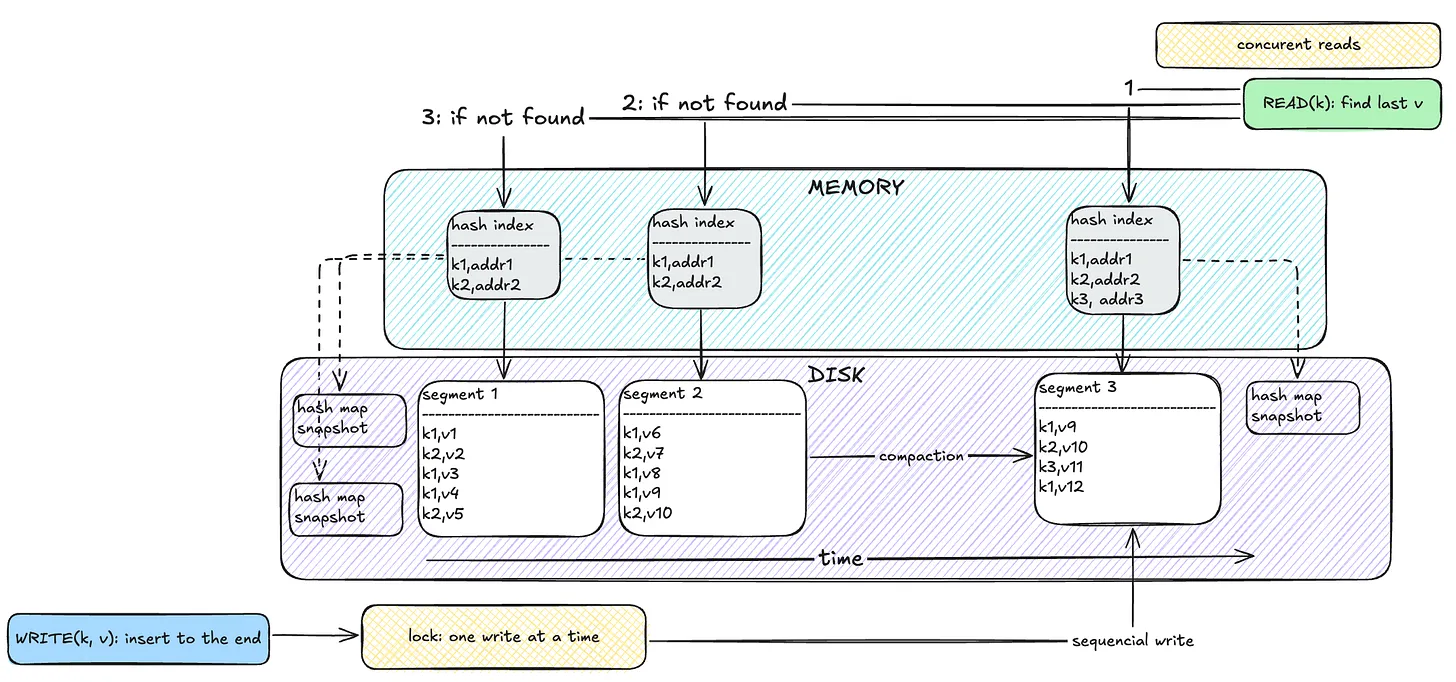
The first simple solution is to make an append-only file and append every pair of keys and values to that file. The read mechanism then scans the whole file and returns the last existing value for the key. The problem is, this can get very slow as the database grows in size because it needs to scan everything. On the other hand, writes are pretty fast since they are sequential rather than random.
To tackle this, we can use memory to store keys and references to the last value on disk. This speeds up reads and adds only a small cost to writes (updating the memory). This is called a hash index. One issue with this approach is that the database size keeps growing, as it doesn’t remove old values.
To improve on that, we can segment the database. Each segment stores key-value pairs up to a certain size, and once full, a new segment is created. A background process called compaction scans segments, keeps only the latest values, and removes outdated ones. This way, the database doesn’t grow indefinitely. Each segment has its own hash index, and reads check the most recent segment first, moving backward if the key isn’t found.
To ensure durability, we can generate hash indexes by scanning segments and storing them in memory at startup. But this makes boot-up time slow. A better approach is to periodically store snapshots of the hash index on disk.
One major issue with this architecture is that it can only hold as many keys as fit in memory. It’s useful when the number of keys is low but values are frequently updated. Examples of databases using this design include Bitcask, Riak, BadgerDB, and Apache Pulsar BookKeeper. Another downside is that range queries (like a < key < b) are very slow because you need to scan all segments.
SSTable and LSM Tree
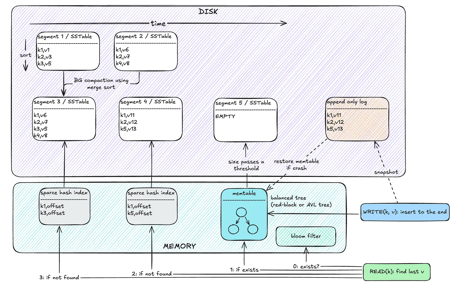
The main limitation of the previous approach was that database capacity was limited by memory size, since we stored all keys in memory. This approach improves that by storing only a selected set of keys in memory, assuming the keys are sorted on disk. To find a key, you locate the greatest key less than or equal to it, and the smallest key greater than it, and scan the range in between.
A memtable is a balanced tree data structure (e.g. red-black or AVL tree) stored in memory. Each write goes to the memtable. When the memtable reaches a size threshold, it’s flushed to disk in a sorted format, and a new memtable is created. Reads first check the memtable, then move through disk segments from most recent to oldest.
Like before, it uses compaction to reduce disk size. Since data in segments is sorted, merge sort can be used to compact and merge them efficiently.
If a key does not exist, you would still need to check the memtable and all segments to be sure. This is improved by adding a Bloom filter—a probabilistic data structure that tells whether a key definitely does not exist or might exist. This helps skip unnecessary scans. Note that bloom filters have false positives, but no false negatives.
Durability is added by periodically storing memtable snapshots to disk. On crash, you can reload the snapshot into memory.
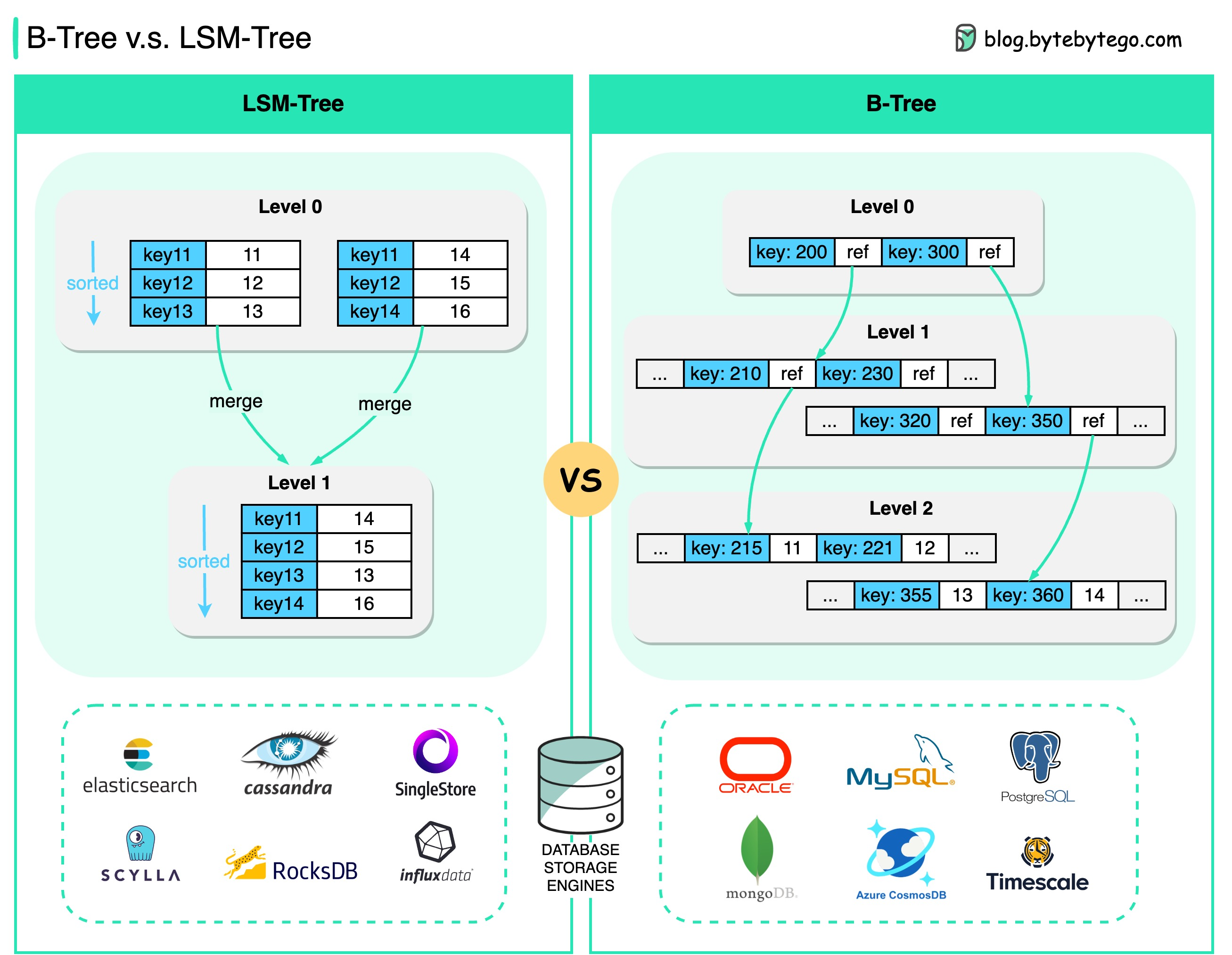
LSM trees are popular for write-heavy databases. Examples include Cassandra, RocksDB, HBase, LevelDB, ScyllaDB, and InfluxDB. The key advantage over B-trees (next section) is that writes happen in memory and are flushed to disk in the background, making writes faster. Reads, however, are slower because they require checking multiple locations (memtable + segments). Compared to the log-structured hash index, LSM trees solve the memory size limitation and support range queries thanks to sorted storage.
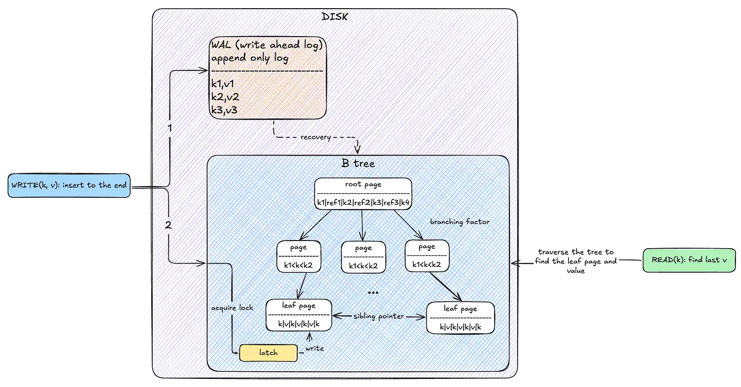
B-trees
Another common data structure used in databases is Balanced Trees. Each node (called a page) is stored at a fixed disk location. Each page contains n+1 keys and n references to child nodes (except for leaf nodes). A child node’s keys are between its parent’s adjacent keys. Searching in an n-node B-tree has a time complexity of O(log n), which is fast.
The downside is that even small changes require overwriting the entire page on disk. To make writes crash-resilient, databases use a WAL (Write-Ahead Log)—writes go here first, then to the B-tree. An alternative is copy-on-write, where a new page is written and then linked, instead of modifying the original (used in filesystems like btrfs).
Compared to LSM trees: - B-trees are generally faster for reads, as each key exists in only one place. - Slower for writes due to random access, full-page rewrites, and dual writes (WAL + page). - B-trees offer better transactional semantics. - B-trees are ideal for read-heavy workloads
Famous databases that use B-trees include PostgreSQL, MySQL (InnoDB), SQLite, Oracle, and SQL Server.
secondary index
So far, we’ve covered how primary indexes work and how they help find items based on exact key matches or range queries. These indexes are designed to retrieve data using the primary key (such as an id or unique identifier).
However, there are many real-world scenarios where we need to look up records based on attributes other than the primary key. This is where secondary indexes come in.
Here are a few examples:
- Finding a user by their email address (a unique secondary index)
- Fetching all orders associated with a user ID (a foreign key index)
- Retrieving all products marked as out-of-inventory (a single-column index)
- Searching for people by first name and last name together (a concatenated index)
- Locating the closest restaurant to a given location using latitude and longitude (multi-dimensional index)
- Matching a user query to the most relevant content or string (full-text search or fuzzy matching index)
Some of these use cases can be handled using data structures similar to primary indexes. For example:
- A unique secondary index behaves much like a primary index but is built on a different column (like
email). - A column index can store multiple matching entries for a given value. This differs from a primary index, which assumes uniqueness. Instead of pointing to a single row, it returns a list of matching rows.
Others require different structures or strategies entirely:
- Foreign key indexes may point from one table’s column to another table’s primary key.
- Geospatial queries (e.g., nearest neighbors) often rely on R-trees which are better suited for multi-dimensional data.
- Full-text search typically uses inverted indexes or fuzzy indexing techniques to match text efficiently, even with typos or variations.
All in all, understanding how different indexing models work—whether it’s log-structured storage with hash indexes, SSTables with LSM Trees, or B-trees—gives you a deeper appreciation of the trade-offs databases make under the hood. Each approach is designed with different performance characteristics in mind, depending on the read/write patterns and use cases. Secondary indexes build on these foundations to support more flexible queries. I hope this post helped shed light on these internal mechanisms, and maybe inspired you to dig deeper into how your favorite databases really work.